BioAlpha Tutorial
In this notebook, we introduce a simple turtorial to do some typical tasks with our library: bioalpha.
This notebook includes 3 main parts:
Part 1: loading library and preparing data for running.
Part 2: processing data via
bioalpha.sc.pp.Part 3: some tools with
bioalpha.sc.tland plotting withbioalpha.sc.pl.
1. Prepare
This notebook uses two 1k cells single-cell datasets obtained from 10xGENOMICS. Include:
1k Human PBMCs with TotalSeq™-B Human TBNK Antibody Cocktail, 3’ v3.1
1k Human PBMCs with TotalSeq™-B Human TBNK Antibody Cocktail, 3’ LT v3.1
1.1. Load required library
import bioalpha
1.2. Download data
!wget -P data/datasets/ https://cf.10xgenomics.com/samples/cell-exp/6.0.0/1k_PBMCs_TotalSeq_B_3p/1k_PBMCs_TotalSeq_B_3p_raw_feature_bc_matrix.h5
!wget -P data/datasets/ https://cf.10xgenomics.com/samples/cell-exp/6.0.0/1k_PBMCs_TotalSeq_B_3p_LT/1k_PBMCs_TotalSeq_B_3p_LT_raw_feature_bc_matrix.h5
1.3. Read data
# Read first dataset
adata1 = bioalpha.sc.read_10x_h5("./data/datasets/1k_PBMCs_TotalSeq_B_3p_raw_feature_bc_matrix.h5")
adata1.var_names_make_unique()

# Read second dataset
adata2 = bioalpha.sc.read_10x_h5("./data/datasets/1k_PBMCs_TotalSeq_B_3p_LT_raw_feature_bc_matrix.h5")
adata2.var_names_make_unique()

# Merge 2 datasets
adata = bioalpha.sc.concat([adata1, adata2], label="batch")
adata.obs_names_make_unique()
adata
AnnData object with n_obs × n_vars = 534586 × 36601
    obs: 'batch'
2. Basic processing data
In this notebook, we introduce some basic tasks when processing data. Including:
Basic filter data
Logarithmize - normalized data
Identify highly-variable genes
Correcting data
Scaling data
Dimension reduction
Get subsample
Batch correction
Compute neighborhood
2.1. Basic data filtering
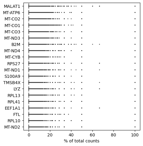
bioalpha.sc.pl.highest_expr_genes(adata, n_top=20,)
bioalpha.sc.pp.filter_cells(adata, min_genes=200)
bioalpha.sc.pp.filter_genes(adata, min_cells=3)
Calculate quality control metrics, annotate mitochodrial genes.
adata.var['mt'] = adata.var_names.str.startswith('MT-')
bioalpha.sc.pp.calculate_qc_metrics(adata, qc_vars=['mt'], percent_top=None, log1p=False, inplace=True)
Filter out cells that have too much mitochondrial genes.
adata = adata[adata.obs.pct_counts_mt < 20, :]
2.2. Logarithmize - normalized data
Normalize each cell by over all genes in order to make the total count of each cell equal after normalization with normalize_total.
The data are also log-transformed with a pseudocount of 1 with log1p.
# bioalpha.sc.pp.normalize_total(adata, target_sum=1e4)
# bioalpha.sc.pp.log1p(adata)
To reduce the execution time, we suggest using log_normalize to do both of those.
bioalpha.sc.pp.log_normalize(adata, target_sum=1e4)
2.3. Identify highly-variable genes
Identify the genes that have highest amount of variance (which are likely to be the most informative).
As bioalpha methods are highly optimized, and can use the whole set of genes to compute, we recommend to use all the genes. The following step is optional.
bioalpha.sc.pp.highly_variable_genes(adata, n_top_genes=2000)
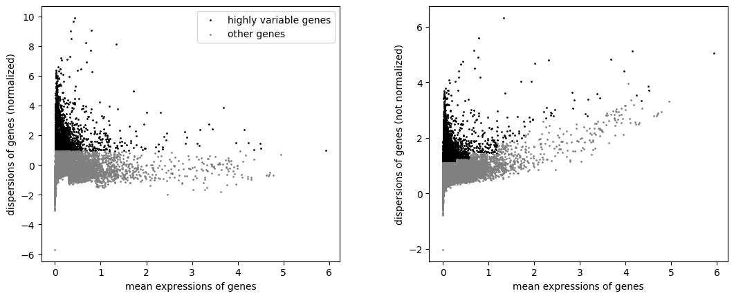
Plot before and after normalization.
bioalpha.sc.pl.highly_variable_genes(adata)
Save data as raw and use high-variable-gene to execute in next step.
If you do not correct data via bioalpha.sc.pp.regress_out and bioalpha.sc.pp.scale, you do not need to save raw data.
adata.raw = adata
adata = adata[:, adata.var.highly_variable]
adata
View of AnnData object with n_obs × n_vars = 1892 × 2000
    obs: 'batch', 'n_genes', 'n_genes_by_counts', 'total_counts', 'total_counts_mt', 'pct_counts_mt'
    var: 'n_cells', 'mt', 'n_cells_by_counts', 'mean_counts', 'pct_dropout_by_counts', 'total_counts', 'highly_variable', 'means', 'dispersions', 'dispersions_norm'
    uns: 'log1p', 'hvg'
2.4. Correcting data
Regress out the effect of unwanted variances (total counts per cell and the percentage of mitochondrial genes expressed).
bioalpha.sc.pp.regress_out(adata, ['total_counts', 'pct_counts_mt'])
adata
AnnData object with n_obs × n_vars = 1892 × 2000
    obs: 'batch', 'n_genes', 'n_genes_by_counts', 'total_counts', 'total_counts_mt', 'pct_counts_mt'
    var: 'n_cells', 'mt', 'n_cells_by_counts', 'mean_counts', 'pct_dropout_by_counts', 'total_counts', 'highly_variable', 'means', 'dispersions', 'dispersions_norm'
    uns: 'log1p', 'hvg'
2.5. Scaling data
Scale each gene to unit variance. Clip values exceeding standard deviation 10.
bioalpha.sc.pp.scale(adata, max_value=10)
2.6. Dimension reduction
Reduce the dimensionality of the data by running principal component analysis (PCA), which reveals the main axes of variation and denoises the data.
With the dataset fewer than 100000 cells, we use the SVD method, otherwise we use History PCA method.
bioalpha.sc.pp.pca(adata, n_comps=50)
WARNING: `data.X` is not spmatrix.To improve performance for further calculations, run `.pp.tosparse` first
WARNING: `data` is ndarray, converting to csr matrix...
2.7. Get sub-sample of data
This step is optional. If the dataset is too large, sub-sampling can improve speed. However, in some cases, it can reduce the accuracy. With highly optimized algorithms in bioalpha, you can run datasets with millions of cells without the need to subsampling the data.
This implementation bases on the Geometric Sketching method.
# bioalpha.sc.pp.subsample(adata, fraction=0.1)
2.8. Batch correction
We use Harmony to integrate different experiments.
In this notebook, the column that differentiates among experiments/batches is "batch".
Change the name of key if it is different in your data.
bioalpha.sc.pp.harmony_integrate(adata, key="batch")
WARNING: `data.X` is not spmatrix.To improve performance for further calculations, run `.pp.tosparse` first
2.9. Compute neighborhood:
Compute the neighborhood graph of cells using the PCA representation of the data matrix by using NNDescent algorithm.
(For results to be similar to Seurat, set n_neighbors to 30, for Scanpy, set n_neighbors to 15).
bioalpha.sc.pp.neighbors(adata, n_neighbors=90, use_rep="X_pca_harmony")
WARNING: `data.X` is not spmatrix.To improve performance for further calculations, run `.pp.tosparse` first
3. Tool and Plot
3.1. Clustering
3.1.1. Kmeans
bioalpha.sc.tl.kmeans(adata, k=10)
WARNING: `data.X` is not spmatrix.To improve performance for further calculations, run `.pp.tosparse` first
3.1.2. Louvain
The louvain implementation directly clusters the neighborhood graph of cells, which we already computed in the previous section.
bioalpha.sc.tl.louvain(adata, resolution=1.0)
WARNING: `data.X` is not spmatrix.To improve performance for further calculations, run `.pp.tosparse` first
3.2. t-SNE
We reimplemnted the following package: FFT-accelerated Interpolation-based t-SNE.
bioalpha.sc.tl.tsne(adata, perplexity=30, use_rep="X_pca_harmony")
WARNING: `data.X` is not spmatrix.To improve performance for further calculations, run `.pp.tosparse` first
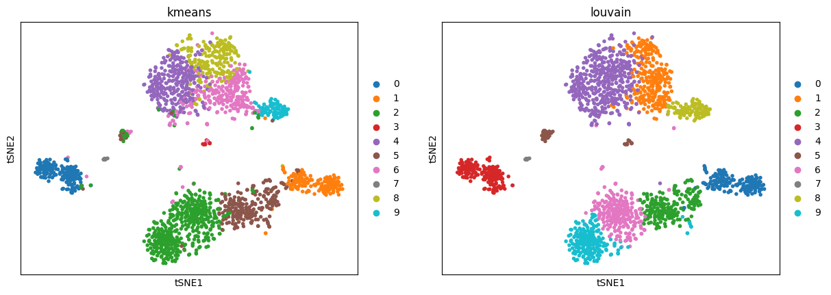
Use bioalpha.sc.pl.tsne to visualize, set color=['louvain'] to color cells only by Louvain cluster labels.
bioalpha.sc.pl.tsne(adata, color=["kmeans", "louvain"])
3.3. UMAP
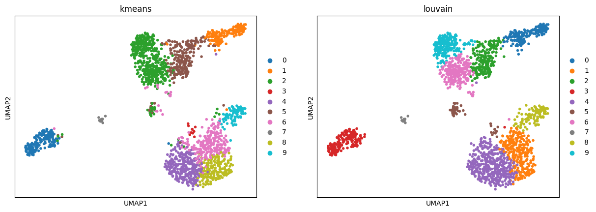
Reducing the dimensionality of our data into two dimensions using uniform manifold approximation (UMAP).
bioalpha.sc.tl.umap(adata, n_components=2, use_rep="X_pca_harmony")
WARNING: `data.X` is not spmatrix.To improve performance for further calculations, run `.pp.tosparse` first
Use bioalpha.sc.pl.umap to visualize, set color=['louvain'] to color cells with only Louvain cluster labels.
bioalpha.sc.pl.umap(adata, color=["kmeans", "louvain"])
3.4. Differential expression
By default, we use “venice”.
bioalpha.sc.tl.rank_genes_groups(adata, groupby="louvain", groups=["3"], method="venice")
WARNING: `data.X` is not spmatrix.To improve performance for further calculations, run `.pp.tosparse` first
Visualize the differential expression in a volcano plot with top highest and lowest "n_genes" log fold changes.
bioalpha.sc.pl.rank_genes_groups_volcano(adata, n_genes=1000)
3.5. Thresholding
bioalpha.sc.experimental.tl.thresholding(adata, groupby="louvain")
WARNING: `data.X` is not spmatrix.To improve performance for further calculations, run `.pp.tosparse` first
3.5. Find marker
Method bioalpha.sc.experimental.tl.find_marker available from version 0.10.0.
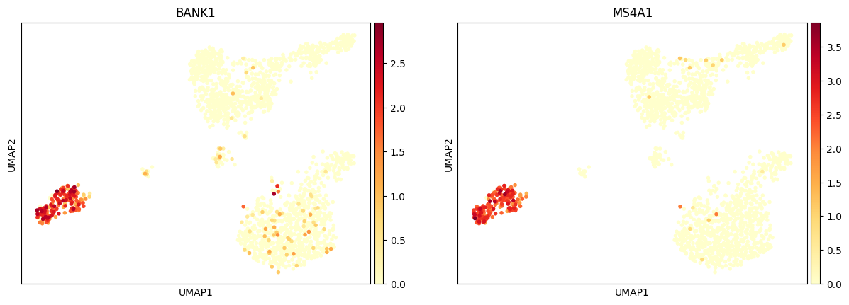
In this example, we find marker genes for cluster "3" in louvain clustering.
A notice that if the groupby is same as the groupby in thresholding, this method will use it to find the genes pannel, otherwise, it will re-compute it.
bioalpha.sc.experimental.tl.find_marker(adata, groupby="louvain", groups=["3"], reference="rest")
WARNING: `data.X` is not spmatrix.To improve performance for further calculations, run `.pp.tosparse` first
Marker genes save on .uns["marker"]["panels"].
adata.uns["marker"]["panels"]["3"]
| possitive | negative | f1_score | |
|---|---|---|---|
| 0 | NIBAN3 | FES | 0.994382 |
| 1 | BANK1, MS4A1 | 0.994382 | |
| 2 | CD79A | 0.991643 | |
| 3 | MS4A1 | 0.991643 | |
| 4 | BANK1, TRBC2 | 0.991597 | |
| 5 | BLK | FES | 0.991597 |
| 6 | BANK1 | NFE2 | 0.991597 |
| 7 | LRRC41, CD79B | 0.991597 | |
| 8 | CD79B | DMXL2 | 0.991597 |
| 9 | BCL11A | RGS18 | 0.991549 |
| 10 | CD79B | S100A6 | 0.991549 |
| 11 | LINC02397 | 0.991549 | |
| 12 | ASPM, IGKC | 0.988889 | |
| 13 | ZBTB17, IGKC | 0.988889 | |
| 14 | RPS27, BANK1 | 0.988827 | |
| 15 | BANK1 | CLEC4E | 0.988827 |
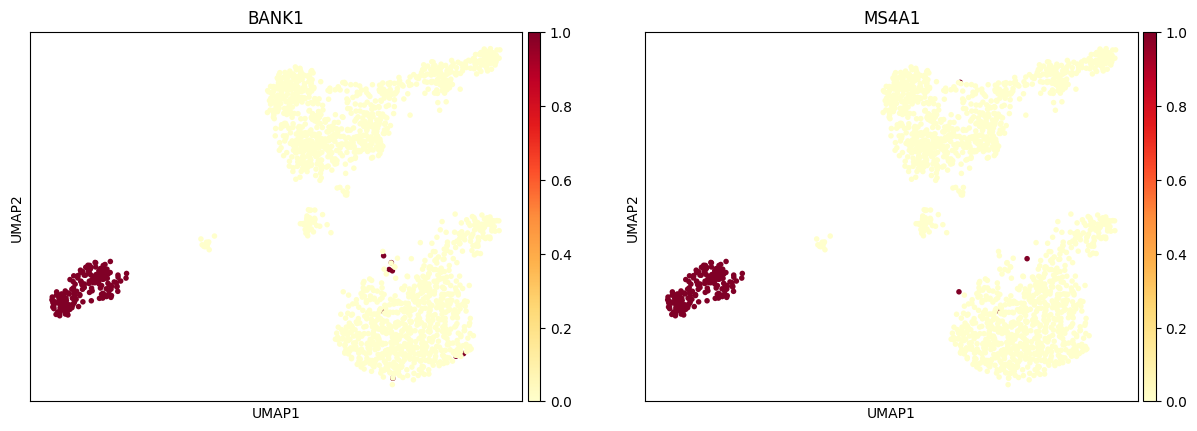
Plot one pair in the gene pannel with UMAP.
bioalpha.sc.pl.umap(adata, color=["BANK1", "MS4A1"], cmap="YlOrRd")
And use the binary_matrix.
bioalpha.sc.pl.umap(adata, color=["BANK1", "MS4A1"], cmap="YlOrRd", layer="binary_matrix", vmin=0, vmax=1)
