BioAlpha Mapping File Tutorial
In this notebook, we introduce a simple turtorial to do some typical tasks with our library: bioalpha.
This notebook includes 3 main parts:
Part 1: loading library and preparing data for running.
Part 2: processing data via
bioalpha.sc.pp.Part 3: some tools with
bioalpha.sc.tland plotting withbioalpha.sc.pl.
1. Prepare
This notebook uses two 1k cells single-cell datasets obtained from 10xGENOMICS. Include:
1k Human PBMCs with TotalSeq™-B Human TBNK Antibody Cocktail, 3’ v3.1
1k Human PBMCs with TotalSeq™-B Human TBNK Antibody Cocktail, 3’ LT v3.1
1.1. Load required library
import bioalpha
1.2. Download data
!wget -P data/datasets/ https://cf.10xgenomics.com/samples/cell-exp/6.0.0/1k_PBMCs_TotalSeq_B_3p/1k_PBMCs_TotalSeq_B_3p_raw_feature_bc_matrix.h5
!wget -P data/datasets/ https://cf.10xgenomics.com/samples/cell-exp/6.0.0/1k_PBMCs_TotalSeq_B_3p_LT/1k_PBMCs_TotalSeq_B_3p_LT_raw_feature_bc_matrix.h5
1.3. Read data
# Read first dataset
adata1 = bioalpha.sc.read_10x_h5("./data/datasets/1k_PBMCs_TotalSeq_B_3p_raw_feature_bc_matrix.h5")
adata1.var_names_make_unique()

# Read second dataset
adata2 = bioalpha.sc.read_10x_h5("./data/datasets/1k_PBMCs_TotalSeq_B_3p_LT_raw_feature_bc_matrix.h5")
adata2.var_names_make_unique()

# Merge 2 datasets
adata = bioalpha.sc.concat([adata1, adata2], label="batch")
adata.obs_names_make_unique()
adata.write_h5ad("./data/datasets/1k_PBMCs_TotalSeq_B_3p.h5ad")
adata = bioalpha.h5ad_map.H5ADMap("./data/datasets/1k_PBMCs_TotalSeq_B_3p.h5ad")
adata
UserWarnings: H5ADMap may write direct to disk. Please backup raw file.
UserWarnings: H5ADMap read data from disk. Please download data to local.
AnnData object with n_obs × n_vars = 534586 × 36601 backed at './data/datasets/1k_PBMCs_TotalSeq_B_3p.h5ad'
    obs: 'batch'
2. Basic processing data
In this notebook, we introduce some basic tasks when processing data. Including:
Basic filter data
Logarithmize - normalized data
Identify highly-variable genes
Correcting data
Scaling data
Dimension reduction
Get subsample
Batch correction
Compute neighborhood
2.1. Basic data filtering
bioalpha.sc.pp.filter_cells(adata, min_genes=200)
bioalpha.sc.pp.filter_genes(adata, min_cells=3)
adata
AnnData object with n_obs × n_vars = 534586 × 36601 backed at './data/datasets/1k_PBMCs_TotalSeq_B_3p.h5ad'
    obs: 'batch', 'n_genes', 'filter_cells_mask'
    var: 'n_cells', 'filter_genes_mask'
Subset data and copy to a new file. It helps us back up raw data.
adata = adata.diet_subset(
    "./data/datasets/1k_PBMCs_TotalSeq_B_3p_processed.h5ad",
    row_index="filter_cells_mask", col_index="filter_genes_mask")
adata
AnnData object with n_obs × n_vars = 2043 × 17447 backed at './data/datasets/1k_PBMCs_TotalSeq_B_3p_processed.h5ad'
    obs: 'batch', 'n_genes', 'filter_cells_mask'
    var: 'n_cells', 'filter_genes_mask'
Calculate quality control metrics, annotate mitochodrial genes.
adata.var['mt'] = adata.var_names.str.startswith('MT-')
bioalpha.sc.pp.calculate_qc_metrics(
    adata, qc_vars=['mt'], percent_top=None, log1p=False, inplace=True)
Filter out cells that have too much mitochondrial genes.
adata.obs["filter_cells_mask"] = adata.obs["pct_counts_mt"] < 20
2.2. Logarithmize - normalized data
Normalize each cell by over all genes in order to make the total count of each cell equal after normalization and also log-transformed with a pseudocount of 1 with log_normalize.
To reduce the execution time, we suggest using log_normalize to do both of those.
bioalpha.sc.pp.log_normalize(
    adata, target_sum=1e4, key_added="X_normalize", obs_mask="filter_cells_mask")
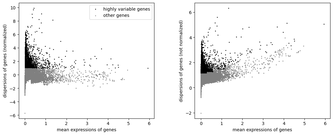
2.3. Identify highly-variable genes
Identify the genes that have highest amount of variance (which are likely to be the most informative).
As bioalpha methods are highly optimized, and can use the whole set of genes to compute, we recommend to use all the genes. The following step is optional.
bioalpha.sc.pp.highly_variable_genes(
    adata, n_top_genes=2000, layer="X_normalize", obs_mask="filter_cells_mask")
Plot before and after normalization.
bioalpha.sc.pl.highly_variable_genes(adata)

Subset adata and save in a new file, we can choose features to keep.
We always keep obs and var of anndata. Anndata.X can be chosen from layers to replace.
adata = adata.diet_subset("./data/datasets/1k_PBMCs_TotalSeq_B_3p_subset.h5ad",
                          X="layers/X_normalize", keys=["uns"],
                          row_index="filter_cells_mask", col_index="highly_variable")
adata
AnnData object with n_obs × n_vars = 1892 × 2000 backed at './data/datasets/1k_PBMCs_TotalSeq_B_3p_subset.h5ad'
    obs: 'batch', 'n_genes', 'filter_cells_mask', 'n_genes_by_counts', 'total_counts', 'total_counts_mt', 'pct_counts_mt'
    var: 'n_cells', 'filter_genes_mask', 'mt', 'n_cells_by_counts', 'total_counts', 'mean_counts', 'pct_dropout_by_counts', 'highly_variable', 'means', 'dispersions', 'dispersions_norm'
    uns: 'hvg', 'log1p'
2.4. Correcting data
Regress out the effect of unwanted variances (total counts per cell and the percentage of mitochondrial genes expressed).
bioalpha.sc.pp.regress_out(
    adata, ['total_counts', 'pct_counts_mt'], key_added="X_regress_out")
<HDF5 dataset "X_regress_out": shape (1892, 2000), type "<f4">
adata
AnnData object with n_obs × n_vars = 1892 × 2000 backed at './data/datasets/1k_PBMCs_TotalSeq_B_3p_subset.h5ad'
    obs: 'batch', 'n_genes', 'filter_cells_mask', 'n_genes_by_counts', 'total_counts', 'total_counts_mt', 'pct_counts_mt'
    var: 'n_cells', 'filter_genes_mask', 'mt', 'n_cells_by_counts', 'total_counts', 'mean_counts', 'pct_dropout_by_counts', 'highly_variable', 'means', 'dispersions', 'dispersions_norm'
    uns: 'hvg', 'log1p'
    layers: 'X_regress_out'
2.5. Scaling data
Scale each gene to unit variance. Clip values exceeding standard deviation 10.
bioalpha.sc.pp.scale(adata, max_value=10, layer="X_regress_out", key_added="X_scale")
adata
AnnData object with n_obs × n_vars = 1892 × 2000 backed at './data/datasets/1k_PBMCs_TotalSeq_B_3p_subset.h5ad'
    obs: 'batch', 'n_genes', 'filter_cells_mask', 'n_genes_by_counts', 'total_counts', 'total_counts_mt', 'pct_counts_mt'
    var: 'n_cells', 'filter_genes_mask', 'mt', 'n_cells_by_counts', 'total_counts', 'mean_counts', 'pct_dropout_by_counts', 'highly_variable', 'means', 'dispersions', 'dispersions_norm'
    uns: 'hvg', 'log1p'
    layers: 'X_regress_out', 'X_scale'
2.6. Dimension reduction
Reduce the dimensionality of the data by running principal component analysis (PCA), which reveals the main axes of variation and denoises the data.
With the dataset fewer than 100000 cells, we use the SVD method, otherwise we use History PCA method.
bioalpha.sc.pp.pca(adata, n_comps=50, layer="X_scale")
We can diet copy and load data without X matrix to memory to optimize running time for other steps.
adata_pca = adata.diet_subset(
    "./data/datasets/1k_PBMCs_TotalSeq_B_3p_subset_pca.h5ad",
    X=None, keys=["obsm/X_pca"])
adata_pca = adata_pca.to_memory()
adata_pca
AnnData object with n_obs × n_vars = 1892 × 2000
    obs: 'batch', 'n_genes', 'filter_cells_mask', 'n_genes_by_counts', 'total_counts', 'total_counts_mt', 'pct_counts_mt'
    var: 'n_cells', 'filter_genes_mask', 'mt', 'n_cells_by_counts', 'total_counts', 'mean_counts', 'pct_dropout_by_counts', 'highly_variable', 'means', 'dispersions', 'dispersions_norm'
    obsm: 'X_pca'
2.7. Batch correction
We use Harmony to integrate different experiments.
In this notebook, the column that differentiates among experiments/batches is "batch".
Change the name of key if it is different in your data.
bioalpha.sc.pp.harmony_integrate(adata_pca, key="batch")
2.8. Compute neighborhood:
Compute the neighborhood graph of cells using the PCA representation of the data matrix by using NNDescent algorithm.
(For results to be similar to Seurat, set n_neighbors to 30, for Scanpy, set n_neighbors to 15).
bioalpha.sc.pp.neighbors(adata_pca, n_neighbors=90, use_rep="X_pca_harmony")
3. Tool and Plot
3.1. Clustering
3.1.1. Kmeans
bioalpha.sc.tl.kmeans(adata_pca, k=10)
3.1.2. Louvain
The louvain implementation directly clusters the neighborhood graph of cells, which we already computed in the previous section.
bioalpha.sc.tl.louvain(adata_pca, resolution=1.0)
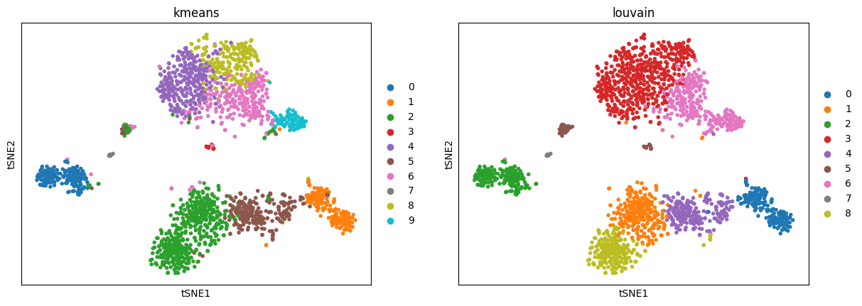
3.2. t-SNE
We reimplemnted the following package: FFT-accelerated Interpolation-based t-SNE.
bioalpha.sc.tl.tsne(adata_pca, perplexity=30, use_rep="X_pca_harmony")
Use bioalpha.sc.pl.tsne to visualize, set color=['louvain'] to color cells only by Louvain cluster labels.
bioalpha.sc.pl.tsne(adata_pca, color=["kmeans", "louvain"])

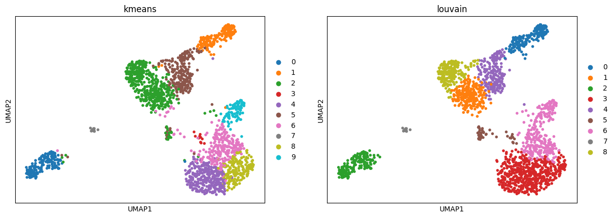
3.3. UMAP
Reducing the dimensionality of our data into two dimensions using uniform manifold approximation (UMAP).
bioalpha.sc.tl.umap(adata_pca, n_components=2, use_rep="X_pca_harmony")
Use bioalpha.sc.pl.umap to visualize, set color=['louvain'] to color cells with only Louvain cluster labels.
bioalpha.sc.pl.umap(adata_pca, color=["kmeans", "louvain"])

3.4. Differential expression
By default, we use “venice”.
adata.obs["louvain"] = adata_pca.obs["louvain"]
bioalpha.sc.tl.rank_genes_groups(
    adata, groupby="louvain", groups=["2"], method="venice", use_raw=False)
adata
AnnData object with n_obs × n_vars = 1892 × 2000 backed at './data/datasets/1k_PBMCs_TotalSeq_B_3p_subset.h5ad'
    obs: 'batch', 'n_genes', 'filter_cells_mask', 'n_genes_by_counts', 'total_counts', 'total_counts_mt', 'pct_counts_mt', 'louvain'
    var: 'n_cells', 'filter_genes_mask', 'mt', 'n_cells_by_counts', 'total_counts', 'mean_counts', 'pct_dropout_by_counts', 'highly_variable', 'means', 'dispersions', 'dispersions_norm'
    uns: 'hvg', 'log1p', 'pca', 'rank_genes_groups'
    obsm: 'X_pca'
    varm: 'PCs'
    layers: 'X_regress_out', 'X_scale'
Visualize the differential expression in a volcano plot with top highest and lowest "n_genes" log fold changes.
bioalpha.sc.pl.rank_genes_groups_volcano(adata, n_genes=1000)